Calibration · state sampling · SNDR · application outcome

Compute SNDR captures temporal noise and spatial distortion.

Compute SNDR combines temporal noise and state-dependent distortion. The full binary $(\mathbf{w},\mathbf{x})$ space contains $2^{2N}$ pairs. The protocol fixes $\mathbf{w}=\mathbf{1}$ , groups the remaining activation patterns by ideal code, and repeats sampled patterns to estimate both effects.

Raw signalEach ADC column returns codes shaped by gain, offset, noise, and row-dependent distortion.

ProtocolCalibrate per column, sample 30 states per ideal code, and repeat every state 10 times.

MetricWeight code-conditioned residual error by $P_{\mathcal Y}(c)$ and compare it with ideal-output variance.

01 · Per-column calibration

Calibrate gain and offset before attributing residual error.

Raw 6-bit ADC output $\widehat y_j$ is mapped to the ideal dot product $y_{\mathrm{o}}$ with an affine MMSE fit computed off-chip for each physical ADC column $j$ . SEC-on evaluation additionally applies the learned output normalization $\theta_j$ .

\widetilde y_j=\theta_j(a_j\widehat y_j+b_j)

MMSE fit	$(a_j,b_j)=\arg\min_{a,b}\sum_{r\in\mathcal D_{\mathrm{cal}}}\left[y_{\mathrm{o},r}-(a\widehat y_{j,r}+b)\right]^2$
Gain	$a_j=\frac{\operatorname{Cov}(y_{\mathrm{o}},\widehat y_j)}{\operatorname{Var}(\widehat y_j)}$
Offset	$b_j=\mathbb{E}[y_{\mathrm{o}}]-a_j\mathbb{E}[\widehat y_j]$
SEC off	$\theta_j=1$
SEC on	$\theta_j$ is the SEC output normalization declared for the measured configuration.

Calibration split

Fit $a_j$ and $b_j$ with $\theta_j=1$ on designated calibration records, freeze the coefficients, then apply the declared SEC-on $\theta_j$ and score evaluation records. The result retains the fit population, column ID, configuration digest, coefficients, units, and analysis commit.

02 · State-space reduction

Sample configurations within every ideal output code.

A binary $N$ -dimensional dot product has $2^{2N}$ joint weight/input configurations. Fixing $\mathbf{w}=\mathbf{1}$ leaves $2^N$ activation patterns over $N+1$ reachable ideal codes. The protocol samples up to $M=30$ activation states per code and repeats every state $K=10$ times.

\left|\{-1,+1\}^{N}\times\{-1,+1\}^{N}\right|=2^{2N},\qquad \mathbf{w}=\mathbf{1}\Rightarrow 2^N\ \text{activation patterns}

\mathcal Y_N=\{-N,-N+2,\ldots,N\},\qquad |\mathcal Y_N|=N+1

Why states matter

For a symbolic four-row example, $\mathbf{x}^{(1)}=[+1,+1,-1,-1]$ and $\mathbf{x}^{(2)}=[+1,-1,+1,-1]$ both produce the ideal code $c=0$ . They activate different physical row patterns, so their $\alpha$ -weighted array currents, and therefore their raw ADC codes, can differ. Sampling states inside one code measures that spatial distortion.

Ideal code

c

Group equal arithmetic outputs

Many physical row patterns map to the same ideal dot-product code.

30 states per codeSample spatial distortion

Different active-row locations expose the $\alpha$ -dependent variation inside one code.

10 repeats per stateSample temporal noise

Repeated evaluation separates within-state noise from pattern-to-pattern distortion.

Protocol scale calculator

Defaults show the nominal $N=64$ protocol scale over $|\mathcal Y_{64}|=65$ reachable signed dot-product codes and eight measured ADC columns.

States per code Repeats per state Reachable codes ADC columns

300measurements per code per column

19,500measurements per column

156,000total captures

\mathcal N_{\mathrm{captures}}=M K|\mathcal C|N_C=30\cdot10\cdot65\cdot8=156{,}000

WITHIN STATE

Repeated noise

Ten captures of the same state expose temporal variation without conflating it with spatial pattern dependence.

WITHIN CODE

Pattern distortion

Thirty distinct row patterns with the same ideal result expose parasitic location dependence.

ACROSS CODES

Operating range

Code-conditioned MSE is weighted by the assumed ideal-output distribution to form column SNDR.

03 · Compute SNDR

Compute one error distribution per ideal code, then weight across codes.

For each ideal code $c$ , squared residuals of calibrated output $\widetilde y_j$ are averaged over states and repeats. Column SNDR uses the same normalized $P_{\mathcal Y}(c)$ in the ideal-output variance and the weighted sum of code-conditioned errors.

P_{\mathcal Y}(c)=2^{-N}\binom{N}{(N+c)/2},\qquad c\in\mathcal Y_N

\operatorname{MSE}_{\mathrm{code},j}(c)=\frac{1}{M_cK}\sum_{s=1}^{M_c}\sum_{k=1}^{K}\left(\widetilde y_{j,c,s,k}-c\right)^2

\operatorname{SNDR}_{\mathrm{col},j}^{(\mathrm{lin})}=\frac{\operatorname{Var}_{P_{\mathcal Y}}(Y_{\mathrm{o}})}{\sum_{c\in\mathcal Y_N}P_{\mathcal Y}(c)\operatorname{MSE}_{\mathrm{code},j}(c)}

\operatorname{SNDR}_{\mathrm{col},j}^{(\mathrm{dB})}=10\log_{10}\!\left(\operatorname{SNDR}_{\mathrm{col},j}^{(\mathrm{lin})}\right)

Result record must include

Dot-product dimension $N$ and reachable code set $\mathcal Y_N$ .
Weight policy, state-selection seed, states per code, and repeats per state.
ADC precision, column IDs, voltage, clock, and operating mode.
Calibration split and per-column gain/offset/normalization.
Ideal-code probability model $P_{\mathcal Y}(c)$ .
SEC state/version and whether learning or inference was active.
Raw-data and analysis-code checksums.

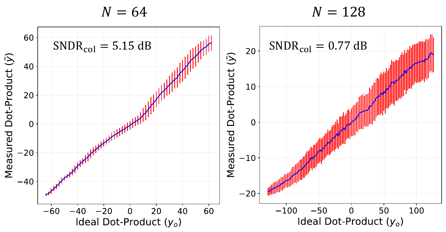
Noise + distortion

The repeated-state protocol makes the two contributions explicit inside each ideal code.

\mathbb E_{s,k}\!\left[(\widetilde y-c)^2\right]=\underbrace{\mathbb E_s\!\left[\operatorname{Var}_k(\widetilde y\mid s)\right]}_{\text{temporal noise}}+\underbrace{\mathbb E_s\!\left[\left(\mathbb E_k[\widetilde y\mid s]-c\right)^2\right]}_{\text{state-dependent distortion}}

Measured MRAM ADC outputs with one-sigma error bars across ideal dot-product codes for dimensions 64 and 128 — **Code-dependent error.** Calibrated output distributions broaden and distort across the operating range. A single RMS value from one input pattern would miss this structure.

Measured silicon

SEC improves the quality–energy operating frontier.

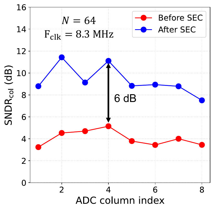
The measured points expose three relationships: increasing $N$ lowers baseline SNDR, SEC raises SNDR across operating conditions, and that gain shifts the iso-SNDR energy point.

Silicon · SEC off

Scaling penalty

$5.15\,\mathrm{dB}$ → $0.77\,\mathrm{dB}$

$N=64\rightarrow N=128$ . Longer active paths increase wire loss and noise.

Silicon ·

N=64

· 8 columns

SEC correction

$4\,\mathrm{dB}$ → $9.15\,\mathrm{dB}$

Average across eight ADC columns. $+2.7\text{–}6\,\mathrm{dB}$ across evaluated operating points.

Silicon · iso-SNDR

Energy frontier

$5\times$ toone fifth

$E_{\mathrm{1bOP,new}}=E_{\mathrm{1bOP,base}}/5$ at iso-SNDR. SEC energy overhead is $0.8\%$ at $N=64$ and $1.8\%$ at $N=128$ .

Implemented / projection

Area implementation

$12.2\%$ → $3.7\%$

Implemented register-based SEC overhead and projected SRAM-backed storage overhead.

Measured SNDR across eight ADC columns before and after statistical error compensation — **Across-column result.** At $N=64$ , the journal reports average SNDR increasing from $4\,\mathrm{dB}$ to $9.15\,\mathrm{dB}$ across eight measured columns.

Application experiment

SEC recovers $7.2$ accuracy points in the measured ResNet-20 output layer.

Software evaluates the convolutional backbone. The macro computes the 4-bit final fully connected layer for 1,000 CIFAR-10 inputs quantized to 7 bits. The same mapping is measured with SEC off and on, with application weights fixed. Hardware results report $\pm5$ percentage points at $90\%$ confidence.

Digital reference

$91.1\%$

Silicon · SEC off

$(74.8\pm5.0)\%$

Silicon · SEC on

$(82.0\pm5.0)\%$

Observed effect

SEC raises top-1 accuracy from 74.8% to 82.0%, so $\Delta A=82.0-74.8=7.2$ percentage points are recovered toward the 91.1% fixed-point digital reference.

Runnable method demo

Run the analysis pipeline on deterministic data.

The repository’s standard-library Python package generates deterministic protocol requests, fits independent affine calibration per column, computes code-conditioned SNDR, and demonstrates an illustrative correction-factor learner on synthetic data.

Run the method demo

Synthetic fixture

The runnable example reports protocol counts, calibration coefficients, and SNDR from generated inputs. The measured result panels above report the ESSCIRC 2023 and JSSC 2025 silicon data.